In the first post we looked at what XPLORE can do and how it can help identify the impact of CBO fixes/parameters but there was no reference to how the tool actually works so let’s try to fix that.

After installing XPLORE using sqlt/utl/xplore/install.sql we need to create our driver script using create_xplore_script.sql, at this point we are already connected as the target user (the installation connects us).
If we need a specific CBO environment now it’s the time to set all the parameters we need, right before starting create_xplore_script.sql.
Let’s keep it simple and assume the default configuration is enough (this holds true most of the times anyway).

Installation completed.
You are now connected as mpagano.

1. Set CBO env if needed
2. Execute @create_xplore_script.sql

SQL> @create_xplore_script.sql

Parameter 1:
XPLORE Method: XECUTE (default) or XPLAIN
"XECUTE" requires /* ^^unique_id */ token in SQL
"XPLAIN" uses "EXPLAIN PLAN FOR" command
Remember EXPLAIN PLAN FOR does not perform bind peeking
Enter "XPLORE Method" [XECUTE]: 

Parameter 2:
Include CBO Parameters: Y (default) or N
Enter "CBO Parameters" [Y]: 

Parameter 3:
Include Exadata Parameters: Y (default) or N
Enter "EXADATA Parameters" [Y]: 

Parameter 4:
Include Fix Control: Y (default) or N
Enter "Fix Control" [Y]: 

Parameter 5:
Generate SQL Monitor Reports: N (default) or Y
Only applicable when XPLORE Method is XECUTE
Enter "SQL Monitor" [N]: 


Review and execute @xplore_script_1.sql

Depending on the values we select at this stage then XPLORE will either execute (XECUTE) or gather an EXPLAIN PLAN FOR (XPLAIN) our SQL, for all the CBO and Exadata parameters and Fix Controls, collecting SQL Monitor reports.

The create script first captures the current CBO environment to use it as baseline and then creates the instructions for each test that will be executed.
Each test looks like

CONN ^^connected_user./^^user_password.^^connect_identifier.
EXEC xplore.set_baseline(1);
ALTER SESSION SET "_fix_control" = '8274946:0';
ALTER SESSION SET STATISTICS_LEVEL = ALL;
DEF unique_id = "xplore_{001}_[^^run_id.]_(00753)"
@^^script_with_sql.
WHENEVER SQLERROR CONTINUE;
ALTER SESSION SET "_fix_control" = '8274946:1';
EXEC xplore.snapshot_plan('xplore_{001}_[^^run_id.]_(00753)', 'XECUTE', 'N');

The first instruction reconnects to make sure we “start fresh” each time.
Then we set the CBO environment to our baseline and set statistics_level =’ALL’ to capture execution statistics.
At this point we can make the change we want to test, in the example above is to turn off the fix for bug 8274946.
Next step is to run our SQL (the unique identifier makes the SQL parsed and helps in identifying the cursor) and once the execution completes then XPLORE captures statistics about the current test from V$SQL, V$SQL_PLAN and V$SQL_PLAN_STATISTICS_ALL storing them into the XPLORE repository tables (tables stored in the target user schema).

In summary SQLT XPLORE iterates over each single CBO/Exadata parameters/Fix Control, changes its value (for some parameters we have several values to test) and capture statistics for the plan generated with such change in place.

After all the tests have been performed XPLORE generates a HTML report with several aggregations starting with a very aggregated overview of the results to then drill little by little up to the final plan with execution statistics for each single test

When upgrading a database sometime you find that one or more SQLs run slower because of a new and suboptimal execution plan. Usually the number of those SQLs is pretty small compared to the overall workload but it’s not straightforward to understand what caused the plan change so even a small number can become tricky to track down.
Each optimizer fix as well as any new feature could be responsible for the plan change but every patchset introduces quite a lot of fixes/features (just check V$SYSTEM_FIX_CONTROL to get an idea) so how can we find out which specific fix is responsible for our performance regression?

The first good news is that CBO fixes are (usually) tied to the OPTIMIZER_FEATURES_ENABLE (OFE) parameter so we can quickly set this param back to the version of the database we upgraded from and check if the SQL returns to the old good performance.
Assuming the answer is yes then the second good news is SQLT provides a way to evaluate each fix_control and CBO parameter, SQLT XPLORE.

XPLORE is an independent module of SQLT that is available under sqlt/utl/xplore, it does require a very small installation (details in the readme.txt) and can be easily removed after our run is complete.
Let’s play a little with XPLORE to better understand its potential and application.

I have a SQL that regressed in performance after a 11.2.0.3 -> 11.2.0.4 upgrade, the SQL is

select count(*)
  from t1, t2, t3
 where t1.id = t2.id
   and t3.store_id = t2.store_id
   and lower(t1.name) like :b1
   and t1.country=:b2
   and t3.store_id = :b3
   and t1.flag=:b4

and the execution plan after the upgrade (right after parse so no possibility bind peeking is trickying us) is

Plan hash value: 1584518234

--------------------------------------------------------------------------------
| Id  | Operation                          | Name         | Rows  | Cost (%CPU)|
--------------------------------------------------------------------------------
|   0 | SELECT STATEMENT                   |              |       |   395 (100)|
|   1 |  SORT AGGREGATE                    |              |     1 |            |
|   2 |   NESTED LOOPS                     |              |     1 |   395  (11)|
|   3 |    NESTED LOOPS                    |              |  6702 |   395  (11)|
|   4 |     TABLE ACCESS BY INDEX ROWID    | T2           |     1 |     2   (0)|
|*  5 |      INDEX RANGE SCAN              | T2_STORE_IDX |     1 |     1   (0)|
|   6 |     BITMAP CONVERSION TO ROWIDS    |              |       |            |
|   7 |      BITMAP AND                    |              |       |            |
|   8 |       BITMAP CONVERSION FROM ROWIDS|              |       |            |
|*  9 |        INDEX RANGE SCAN            | T1_ID_IDX    |  6702 |    18   (6)|
|  10 |       BITMAP CONVERSION FROM ROWIDS|              |       |            |
|  11 |        SORT ORDER BY               |              |       |            |
|* 12 |         INDEX RANGE SCAN           | T1_FLAG_IDX  |  6702 |   103   (6)|
|* 13 |    TABLE ACCESS BY INDEX ROWID     | T1           |     1 |   395  (11)|
--------------------------------------------------------------------------------

Predicate Information (identified by operation id):
---------------------------------------------------
   5 - access("T2"."STORE_ID"=:B3)
   9 - access("T1"."ID"="T2"."ID")
  12 - access("T1"."FLAG"=:B4)
       filter("T1"."FLAG"=:B4)
  13 - filter((LOWER("T1"."NAME") LIKE :B1 AND "T1"."COUNTRY"=:B2))

Note T3 is removed by Join Elimination transformation
The plan cost is pretty small because the estimation for step 12 is very off and the real number of rows returned on such step is over 90% of the data, making the performance drop significantly.
Setting OFE back to 11.2.0.3 then the old good plan is generated

Plan hash value: 2709605153

----------------------------------------------------------------------------
| Id  | Operation                      | Name         | Rows  | Cost (%CPU)|
----------------------------------------------------------------------------
|   0 | SELECT STATEMENT               |              |       |  2007 (100)|
|   1 |  SORT AGGREGATE                |              |     1 |            |
|   2 |   NESTED LOOPS                 |              |   354 |  2007   (2)|
|   3 |    NESTED LOOPS                |              |  6702 |  2007   (2)|
|   4 |     TABLE ACCESS BY INDEX ROWID| T2           |     1 |     2   (0)|
|*  5 |      INDEX RANGE SCAN          | T2_STORE_IDX |     1 |     1   (0)|
|*  6 |     INDEX RANGE SCAN           | T1_ID_IDX    |  6702 |    18   (6)|
|*  7 |    TABLE ACCESS BY INDEX ROWID | T1           |   332 |  2005   (2)|
----------------------------------------------------------------------------

Predicate Information (identified by operation id):
---------------------------------------------------
   5 - access("T2"."STORE_ID"=:B3)
   6 - access("T1"."ID"="T2"."ID")
   7 - filter((LOWER("T1"."NAME") LIKE :B1 AND "T1"."COUNTRY"=:B2 AND
      "T1"."FLAG"=:B4))

Here the cost is more realistic and the CBO stayed away from T1_FLAG_IDX so the final performance is much better

We have one of those cases where after an upgrade the SQL runs slow and setting OFE back to the previous version reverts the old good plan, let’s see how XPLORE is going to help us find out what changed my plan.

In my specific case I reproduced both plans in a test environment where I have no data (took 3 mins to reproduce thanks to a SQLT TC 😉 so even the poor plan will not take more than a few milliseconds to run, just the parse time.

To install XPLORE all we need to do is connect as SYS, run install.sql and provide the username/pwd of the user we want to run XPLORE from. In case our system runs with a non default CBO environment and we need it to replicate the plans then we will be asked to set the proper environment too so that XPLORE can define a baseline CBO environment.
At the end of the installation a file called xplore_script_1.sql is generated, that’s our XPLORE driver script.

Next step is to run XPLORE so let’s connect as our application user and start xplore_script_1.sql
Input parameters are the name of the script for our SQL (remember the mandatory /* ^^unique_id */ comment!!!) and the password for our application user.

SQL> @xplore_script_1.sql

CONNECTED_USER
------------------------------
TC84168

Parameter 1:
Name of SCRIPT file that contains SQL to be xplored (required)
Note: SCRIPT must contain comment /* ^^unique_id */

Enter value for 1: myq.sql

Parameter 2:
Password for TC84168 (required)

Enter value for 2:

At this point XPLORE will test all the fix_controls and CBO parameters generating an execution plan for each of them (for some parameters, ie. optimizer_index_cost_adj we test several values), packing the result in a HTML report.

Let’s navigate the result

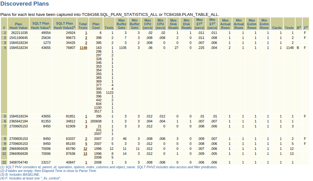
The section reports a list of all the PHVs identified, how many tests generated each plan as well as other useful information about those plans (some details later).
Looks like both are good (PHV 2709605153) and bad (PHV 1584518234) execution plans have been reproduced so let’s focus our attention on those two in the next section

We see that for our bad plan there are three lines, same PHV but different SQLT PHVs, that’s because those two additional PHVs are more restrictive and take into consideration additional factors (ie. filters) to better help differentiate between plans.
The plan in line #3 has been generated by 1148 tests including our baseline (‘B’) “execution zero” that is with no parameter/fix_control change. It’s not surprising to have so many tests generating the same plan as the baseline because most of the fixes/params usually don’t affect each and every SQL.

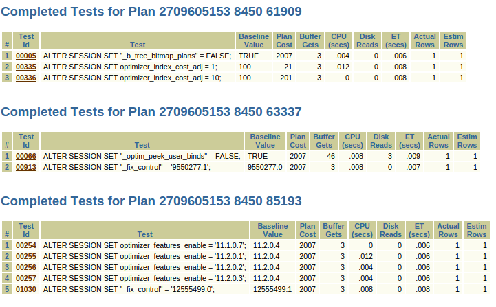
Our target plan is the one reported at lines #7,8,9 so let’s navigate to them

That’s the list of all the parameters and fix_controls that can lead to our good plan so we just need to go back to MOS and get some more information about those fixes to decide which one we want to test.
In this case the answer is 12555499 because it generates the same identical plan as OFE=11.2.0.3.

It’s usually better to use a fix_control rather than a parameter since the former is more likely to have a narrower scope than the latter.

SQL> alter session set "_fix_control"='12555499:0';
Session altered.

SQL> @myq
PL/SQL procedure successfully completed.
PL/SQL procedure successfully completed.
PL/SQL procedure successfully completed.
PL/SQL procedure successfully completed.

  COUNT(*)
----------
	 0

Plan hash value: 2709605153

----------------------------------------------------------------------------
| Id  | Operation                      | Name         | Rows  | Cost (%CPU)|
----------------------------------------------------------------------------
|   0 | SELECT STATEMENT               |              |       |  2007 (100)|
|   1 |  SORT AGGREGATE                |              |     1 |            |
|   2 |   NESTED LOOPS                 |              |   354 |  2007   (2)|
|   3 |    NESTED LOOPS                |              |  6702 |  2007   (2)|
|   4 |     TABLE ACCESS BY INDEX ROWID| T2           |     1 |     2   (0)|
|*  5 |      INDEX RANGE SCAN          | T2_STORE_IDX |     1 |     1   (0)|
|*  6 |     INDEX RANGE SCAN           | T1_ID_IDX    |  6702 |    18   (6)|
|*  7 |    TABLE ACCESS BY INDEX ROWID | T1           |   332 |  2005   (2)|
----------------------------------------------------------------------------

Predicate Information (identified by operation id):
---------------------------------------------------

   5 - access("T2"."STORE_ID"=:B3)
   6 - access("T1"."ID"="T2"."ID")
   7 - filter((LOWER("T1"."NAME") LIKE :B1 AND "T1"."COUNTRY"=:B2 AND
	      "T1"."FLAG"=:B4))

So using SQLT XPLORE we found in a few minutes which fix changed our execution plan, a workaround with a very narrow scope and also a way to research in MOS if any known issue related to this specific fix has been reported.

SQLT XPLORE can be used to troubleshoot other types of issues too, ie the report shows Min/Max Elapsed Time (ET) per plan as well as the ET per test, in case of no-data testcase then all the time will be parse time so we can use XPLORE to troubleshoot slow-parse issues and find which feature is accounting for most of the time and what to set to reduce such parse time