Mauro Pagano's Blog


Leave a comment

What I forgot and had to relearn about DESC indexes

The title for this blog post is probably more catchy than the post itself but the election is close so every sort of campaign is allowed, right?
This post is another one of those “I knew it, but I forgot and got bitten back” blog post so hopefully next time I see it I’ll be quicker in recognizing such behavior.

The goal of the SQL is to quickly return the Top-N rows  that match some filter condition(s), descendingly sorted by one of such columns. Pretty common requirement if you consider the filter/sort column to be a date one (“give me the last day worth of transactions, starting with the most recent ones”) and many people would solve using a DESC index on the date column.

drop table t purge;

create table t (pk number, owner varchar2(128), object_id number, data_object_id number, created date, object_name varchar2(128), object_type varchar2(23), large_column clob, random_stuff varchar2(20));

insert into t 
 select /*+ LEADING(A) */ rownum pk, a.owner, a.object_id, a.data_object_id, 
        (sysdate-31)+(rownum/65000) created, a.object_name, a.object_type,  
        to_clob(null) large_column, lpad('a',20,'a') random_stuff
   from dba_objects a,
        (select rownum from dual connect by rownum <= 20) b
  where rownum <= 2000000;

exec dbms_stats.gather_table_stats(user,'T');

create index i_desc on t(created desc);

var from_d varchar2(100);
var to_d varchar2(100);
var maxrows number;

exec :from_d := '20161001';
exec :to_d := '20161002';
exec :maxrows := '25';

SELECT data.*, ROWNUM AS rn 
  FROM (SELECT /*+ INDEX(t i_desc) */ * 
          FROM t 
         WHERE created BETWEEN to_date(:from_d,'YYYYMMDD') AND to_date(:to_d,'YYYYMMDD')
         ORDER BY created DESC) data
 WHERE ROWNUM < :maxrows

Plan hash value: 2665129471

--------------------------------------------------------------------------------
| Id  | Operation                      | Name  | Starts | E-Rows|A-Rows|Buffers|
--------------------------------------------------------------------------------
|   0 | SELECT STATEMENT               |       |      1 |       |    24|     50|
|*  1 |  COUNT STOPKEY                 |       |      1 |       |    24|     50|
|   2 |   VIEW                         |       |      1 |     27|    24|     50|
|*  3 |    FILTER                      |       |      1 |       |    24|     50|
|   4 |     TABLE ACCESS BY INDEX ROWID| T     |      1 |  65002|    24|     50|
|*  5 |      INDEX RANGE SCAN          | I_DESC|      1 |      3|    24|     26|
--------------------------------------------------------------------------------

Predicate Information (identified by operation id):
---------------------------------------------------
1 - filter(ROWNUM<:MAXROWS)   
3 - filter(TO_DATE(:TO_D,'YYYYMMDD')>=TO_DATE(:FROM_D,'YYYYMMDD'))
5 - access("T"."SYS_NC00010$">=SYS_OP_DESCEND(TO_DATE(:TO_D,'YYYYMMDD')) AND
           "T"."SYS_NC00010$"<=SYS_OP_DESCEND(TO_DATE(:FROM_D,'YYYYMMDD')))
    filter((SYS_OP_UNDESCEND("T"."SYS_NC00010$")<=TO_DATE(:TO_D,'YYYYMMDD') AND            
            SYS_OP_UNDESCEND("T"."SYS_NC00010$")>=TO_DATE(:FROM_D,'YYYYMMDD')))

Execution plan has no SORT ORDER BY [STOPKEY in case case] thanks to the way values are stored in the index (DESC order) thus no blocking operation. As soon as 24 rows are retrieved from the index/table steps (aka they satisfy the filter conditions) they can be immediately returned to the user.

Your business goes well, data volume increase and so you decide to range partition table T by time and to make partition maintenance smooth you make index I_DESC LOCAL. SQL commands are the same as before except for the PARTITION clause in the CREATE TABLE and the LOCAL keyword in the CREATE INDEX.

drop table t purge;

create table t (pk number, owner varchar2(128), object_id number, data_object_id number, created date, object_name varchar2(128), object_type varchar2(23), large_column clob, random_stuff varchar2(20))
 partition by range (created) interval (numtodsinterval(7,'day')) 
  (partition p1  values less than (to_date('2016-09-12 00:00:00', 'yyyy-mm-dd hh24:mi:ss')));

insert into t 
 select /*+ LEADING(A) */ rownum pk, a.owner, a.object_id, a.data_object_id, 
        (sysdate-31)+(rownum/65000) created, a.object_name, a.object_type,  
        to_clob(null) large_column, lpad('a',20,'a') random_stuff
   from dba_objects a,
        (select rownum from dual connect by rownum <= 20) b
  where rownum <= 2000000;

exec dbms_stats.gather_table_stats(user,'T');

create index i_desc on t(created desc) local;

SELECT data.*, ROWNUM AS rn 
  FROM (SELECT /*+ INDEX(t i_desc) */ * 
          FROM t 
         WHERE created BETWEEN to_date(:from_d,'YYYYMMDD') AND to_date(:to_d,'YYYYMMDD')
         ORDER BY created DESC) data
 WHERE ROWNUM < :maxrows;

-------------------------------------------------------------------------------------------
| Id |Operation                                      |Name   |Starts|E-Rows|A-Rows|Buffers|
-------------------------------------------------------------------------------------------
|   0|SELECT STATEMENT                               |       |     1|      |    24|    855|
|*  1| COUNT STOPKEY                                 |       |     1|      |    24|    855|
|   2|  VIEW                                         |       |     1|    27|    24|    855|
|*  3|   SORT ORDER BY STOPKEY                       |       |     1|    27|    24|    855|
|*  4|    FILTER                                     |       |     1|      | 65001|    855|
|   5|     PARTITION RANGE ITERATOR                  |       |     1| 65002| 65001|    855|
|   6|      TABLE ACCESS BY LOCAL INDEX ROWID BATCHED|T      |     1| 65002| 65001|    855|
|*  7|       INDEX RANGE SCAN                        |I_DESC |     1|     2| 65001|    187|
-------------------------------------------------------------------------------------------

Predicate Information (identified by operation id):
---------------------------------------------------
1 - filter(ROWNUM<:MAXROWS)
3 - filter(ROWNUM<:MAXROWS)  
4 - filter(TO_DATE(:TO_D,'YYYYMMDD')>=TO_DATE(:FROM_D,'YYYYMMDD'))
7 - access("T"."SYS_NC00010$">=SYS_OP_DESCEND(TO_DATE(:TO_D,'YYYYMMDD')) AND
           "T"."SYS_NC00010$"<=SYS_OP_DESCEND(TO_DATE(:FROM_D,'YYYYMMDD')))     
    filter((SYS_OP_UNDESCEND("T"."SYS_NC00010$")>=TO_DATE(:FROM_D,'YYYYMMDD') AND
            SYS_OP_UNDESCEND("T"."SYS_NC00010$")<=TO_DATE(:TO_D,'YYYYMMDD')))

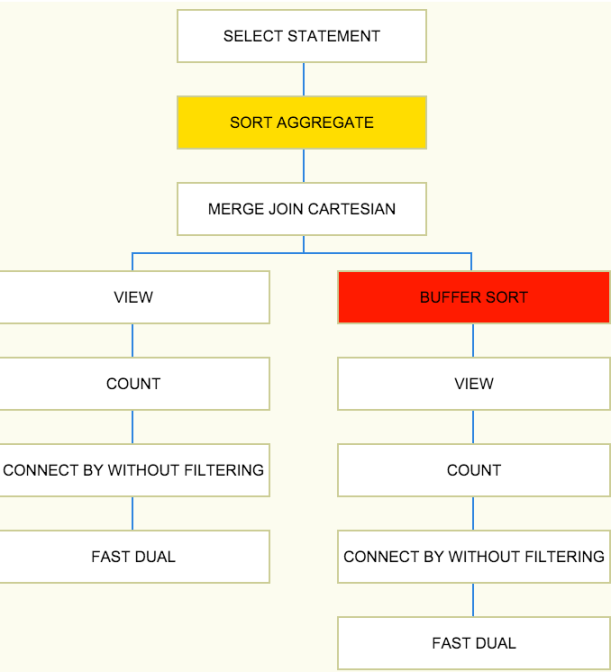
Unfortunately this time the plan DOES include a SORT ORDER BY STOPKEY and the effect is evident, ~65k rows are retrieved before the top 24 are returned back to the user.

Why is that? Let’s hold the question for a second and check first if an ASC index would make a difference here.
Do we have the same behavior if instead of scanning the I_DESC index using a regular “INDEX RANGE SCAN” we do a “INDEX RANGE SCAN DESCENDING” on an index defined as ASC?
Same SQL commands as before except the index is defined ASC and the hint now becomes INDEX_DESC.

create index i_asc on t(created) local;

SELECT data.*, ROWNUM AS rn 
  FROM (SELECT /*+ INDEX_DESC(t i_asc) */ * 
          FROM t 
         WHERE created BETWEEN to_date(:from_d,'YYYYMMDD') AND to_date(:to_d,'YYYYMMDD')
         ORDER BY created DESC) data
 WHERE ROWNUM < :maxrows;

---------------------------------------------------------------------------------------
| Id |Operation                             | Name  |Starts|E-Rows|Pstart|Pstop|A-Rows|
---------------------------------------------------------------------------------------
|   0|SELECT STATEMENT                      |       |     1|      |      |     |    24|
|*  1| COUNT STOPKEY                        |       |     1|      |      |     |    24|
|   2|  VIEW                                |       |     1|    27|      |     |    24|
|*  3|   FILTER                             |       |     1|      |      |     |    24|
|   4|    PARTITION RANGE ITERATOR          |       |     1|    27|  KEY |  KEY|    24|
|   5|     TABLE ACCESS BY LOCAL INDEX ROWID| T     |     1|    27|  KEY |  KEY|    24|
|*  6|      INDEX RANGE SCAN DESCENDING     | I_ASC |     1| 65002|  KEY |  KEY|    24|
---------------------------------------------------------------------------------------

Predicate Information (identified by operation id):
---------------------------------------------------
1 - filter(ROWNUM<:MAXROWS)     
3 - filter(TO_DATE(:TO_D,'YYYYMMDDHH24')>=TO_DATE(:FROM_D,'YYYYMMDD'))
6 - access("CREATED"<=TO_DATE(:TO_D,'YYYYMMDD') AND "CREATED">=TO_DATE(:FROM_D,'YYYYMMDD'))
    filter(("CREATED">=TO_DATE(:FROM_D,'YYYYMMDD') AND "CREATED"<=TO_DATE(:TO_D,'YYYYMMDD')))

Expected plan again, without SORT step, that returns 24 rows as soon as they are extracted from the index/table step.
So to answer the initial question, is there a difference?
Yes, when using a “INDEX RANGE SCAN DESCENDING” of I_ASC index the database didn’t include the SORT step. On the other hand when doing an “INDEX RANGE SCAN” of I_DESC index the SORT step is included and it affects the performance of the SQL.

Why when using the DESC index there is a SORT step?
I can’t imagine why the database needs to introduce that SORT step, beside restriction / limitations in the code (but this is based on limited knowledge so easy to be wrong here).
My guess is the additional complexity of the DESC index code / filters combined with bind variables limit the ability to recognize the SORT is unnecessary.

Reason for saying this it’s anytime Oracle does dynamic partitioning pruning (because of the binds, aka Pstart/Pstop KEY/KEY) the SORT step is present even though such step is not there when using “INDEX RANGE SCAN DESCENDING” on I_ASC index still in presence of binds. Also the SORT disappears when using “INDEX RANGE SCAN” on I_DESC index if the binds are replaced with literals.
One suspect was that the PARTITION RANGE ITERATOR step was consistently being executed in ASCENDING way, if that was the case then the SORT would make sense because the data would be returned “partially” sorted, meaning desc sorted only within each partition. But this is not the case, event 10128 (details here) show the partitions are accessed in DESCENDING order

Partition Iterator Information:
 partition level = PARTITION
 call time = RUN
 order = DESCENDING
 Partition iterator for level 1:
 iterator = RANGE [3, 4]
 index = 4
 current partition: part# = 4, subp# = 1048576, abs# = 4
 current partition: part# = 3, subp# = 1048576, abs# = 3

That’s why the (educated guesssed) conclusion that the SORT step is just caused my some limitations rather than being necessary here, corrections are very welcome here!!!
What just said adds to the very good reasons to question a DESC index on a single column to begin with, reported by Richard Foote here.

BTW apologies for the DDL not super-clean, they were just inherited from another example I was working on and came in handy 😀


2 Comments

Which Observations would you like to see in SQLd360?

SQLd360 v1617 finally includes a new “Observations” section (section 1F) that I pushed back for long, very long 🙂

If you are not familiar with SQLTXPLAIN then consider the reports in this section like “yellow flags”, specific items that are not necessarily causing direct troubles to your SQL but are still questionable and need further investigation / verification / blessing for such item to be kept in place.

There are many reasons why I pushed back for a long time, first one being the results can be easily misleading and make you believe the underlying cause is A while maybe it’s Z. Another reason is most of the observations ended up just being informative with no action taken against them, still you had to scroll hundreds of them.
Because of what just said, combined with the need to keep the checks “useful”, the current list of observations is intentionally short (and incomplete as of now), it includes only observations for:

  • Some system-wide settings, e.g. CBO parameters, OFE version, etc
  • Few plan and cursor-specific information, e.g. index referenced in some plan is now missing
  • Table statistics, e.g. partition that are empty according to stats

The list won’t grow much based on my ideas for the same reason it’s short now, I don’t want to implement checks I believe are important when 99% of the people don’t care about them.

That’s why this blog post, I need your feedback and ideas to implement what you care about 🙂
Let me know what you would like to have in the observation section and I’ll work on it!
Just keep in mind the goal is to keep that section relatively fast so super-complex checks that take 10 mins to execute are off the list.

Note: v1617 also turns off a couple of less-used features like TCB and AWR reports by default (can easily be enabled back via config file) so don’t be surprised if they don’t show up in column 5.


Leave a comment

How to find file and block# to dump in Exadata

Probably because of my past with Oracle Support, I find myself collecting traces and dumps on a regular basis. For example every time I see a row source operation that I would expect to perform only multiblock reads (e.g. Full Table Scan) doing single block ones I collect some block dumps to understand why that is happening. It’s just a matter of looking at the raw SQL trace file (or P1/P2 from ASH for that matter) for the unexpected single block reads, grab file# and block# and dump the block.

Single block reads in Exadata become “cell single block physical read” and the P1/P2 for the wait event don’t show the file#/block# but rather then cellhash# and diskhash# where the data came from. This is a little annoying to me because I can’t just grab cellhash#/diskhash# (plus bytes, that matches with the block size being a single block read) and dump that AS FAR AS I KNOW (corrections are very welcome here).

The way I usually work it around is using with ASM info enabling KFKIO tracing (trace[KFKIO] using the 11g new syntax) before running the “guilty SQL” so that each read now looks like this

...
2016-05-05 19:05:41.351021 : KFK_IODONE_OSS:iop:0x7f1841034000 bufp:0x1124ae000 op:1 au:120555 dsk:0x2 err:1 osderr:0 ossp:0x7f1841166fc8 ossp->errcode_oss_result:(nil) io elapsed time: 0 usec time waited on io: 0 usec
2016-05-05 19:05:41.351052 : kfk_iodone_oss_retry::in iop:0x7f1841034000
2016-05-05 19:05:41.351062 : kfk_iodone_oss_retry::out retry:0
2016-05-05 19:05:41.351071 : KFK:IODONE:iop:0x7f1841034000 wt:1 sstype:1 mastp:(nil) result:1 path:o/192.168.12.5/DATA_CD_01_enkx3cel03 au_offset:2678784 operation:1 reason:3347 iosize:8192 bufp:0x1124ae000
WAIT #139742149463208: nam='cell single block physical read' ela= 346 cellhash#=379339958 diskhash#=3782402265 bytes=8192 obj#=115376 tim=1462493141351085
...

What I care about is:

  • path:o/192.168.12.5/DATA_CD_01_enkx3cel03 -> where the data is stored
  • au:120555 -> the ASM allocation unit where my block is stored in
  • au_offset:2678784 -> how far in the allocation unit my block is

using this info I can go to the ASM instance (reason why ASM instance is becaused  X$KFFXP isn’t exposed in the RDBMS instance) and using the following SQL extract file name and block number

SELECT a.name file_name, 
       xnum_kffxp * (&&au_size./&&db_block_size.) + &&au_offset./&&db_block_size. block_num
  FROM x$kffxp x, 
       v$asm_alias a
 WHERE (x.disk_kffxp, x.group_kffxp) IN (SELECT number_kfdsk, grpnum_kfdsk 
                                           FROM x$kfdsk 
                                          WHERE path_kfdsk = '&&path.')
   AND x.au_kffxp = &&au.
   AND x.number_kffxp = a.file_number
   AND x.incarn_kffxp = a.file_incarnation;

The SQL will ask for 5 parameters, 3 of which are already available while the other two are:

  • au_size -> Allocation Unit size -> V$ASM_DISKGROUP.ALLOCATION_UNIT_SIZE
  • db_block_size -> the DB_BLOCK_SIZE

So for example using the values from above plus 4194304 au_size and 8192 bytes block size the result will be

FILE_NAME                                            BLOCK_NUM
-------------------------------------------------- -----------
USERS.1155.861540195                                   3946823

Disclaimer: the SQL could take a little while since it needs to scan the list of extents.

I know it’s a little convoluted but as of now I haven’t found a more efficient way to identify file/block to dump starting from cellhash#/diskhash#.

Goes without saying I’d love to hear smarter ways to get it done 🙂

UPDATE: Stefan Koehler (who is awesome on top of being a friend) made a very valid point on Twitter, event 10200 can lead to the same info without having to go to the ASM instance. I discarded the event when I started looking at this because it was a little too verbose but then I ended up with KFKIO that is even more verbose!  😦
Stupid me and thanks to Stefan!

An output of event 10200 looks like this

ktrget2(): started for block  0x0005 : 0x05fc3947 objd: 0x0001c2b0
...
WAIT #139650546118344: nam='cell single block physical read' ela= 380 cellhash#=379339958 diskhash#=3782402265 bytes=8192 obj#=115376 tim=1462544482448025

where 05fc3947 is the DBA, 100415815 in decimal, and using DBMS_UTILITY we can extract file and block# from it

SELECT dbms_utility.data_block_address_file(100415815) file_n,
       dbms_utility.data_block_address_block(100415815) block_n
  FROM dual;

    FILE_N    BLOCK_N
---------- ----------
        23    3946823


1 Comment

eAdam, SQLd360 hidden gem

The title is actually VERY wrong! eAdam isn’t a gem hidden inside SQLd360, it’s a standalone tool developed by Carlos Sierra and it’s been around for way longer than SQLd360. You can read more about eAdam here but in short its goal is to export AWR data in a portable way that can be restored in another database, something like a raw version of AWR Warehouse (kind of).

Every time you run SQLd360, the tool collects a reduced version of eAdam just for ASH data (both GV$ and DBA_HIST) for the SQL of interest, packs the result into the zip file and links it into the main page under column 5, “eAdam ASH”. The reason for doing so is SQLd360 has tons of reports built on top of the most important columns of ASH but what if you want to query another column that is not present in any report? With eAdam you basically have the whole ASH for this SQL ID to do all the data mining you want!

I’m writing this post because I realized I never advertised this functionality much and every time I talk about it with somebody, he/she looks at me like “what are you talking about? I’ve never seen it”.

So let me show you how easy it is to load eAdam data coming from SQLd360 into a target database! I’m assuming you already have eAdam installed (if not then just follow the first two steps in “Instructions – Staging Database” from this link)

  1. Grab file NNNN_sqld360_<<hostname_hash>>_<<sql_id>>_5_eadam_ash.tar from inside SQLd360, it will be one of the last files.
  2. Place it into <<path to eAdam>>/stage_system and just run eadam_load.sql as the eAdam user you created during the installation.

Done!

You now have two tables in your eAdam schema called GV_ACTIVE_SESSION_HISTORY_S and DBA_HIST_ACTIVE_SESS_HIST_S with all the ASH data for your SQL ID!


5 Comments

Introducing TUNAs360 – Tuning with Active Sessions without Diagnostic Pack


I’m happy to introduce a new free tool that allows to get initial insights about a database using eDB360/SQLd360 like charts without Diagnostic Pack!!!

(TUN)ing with (A)ctive (s)essions, aka TUNAs360, requires no installation and no parameter when executed; it observes the workload for few minutes and then collects a set of reports on such load.

The idea behind the tool is to help getting started in those situations where there is a concern with database performance but the reason is unknown, the classic “the database is slow but I don’t know why”.
In case further investigation is necessary then eDB360 or SQLd360 can be leveraged.

Once executed TUNAs360 provides several reports for the whole database (cluster and node specific) plus additional reports to help drill into the details of the top 5 sessions and top 5 SQLs during the time the load was observed.

The tool belongs to the “360 family” so it has the same look and many of the charts of its bigger brothers, the main page looks like this

Screen Shot 2016-03-21 at 8.00.05 PM

To execute the tool:

  1. Download the tool from the link on the right side of the screen.
  2. Unzip file tunas360-master.zip
  3. Navigate into tunas360-master folder
  4. Connect as a DBA user and run script tunas360.sql

The tool will run for a few minutes and it will generate a zip file named tunas360_<dbname>_<host>_YYYYMMDD_HH24MI.zip.

As every other tool on its first version I don’t expect it to be perfect so please please please let me know if you run into problems so that I can fix them 😀

Feedbacks and suggestions are welcome as usual too!!!


Leave a comment

Top Executions SQL Monitoring style reports in SQLd360

I think SQL Monitoring is an amazing tool when it comes to SQL Tuning but I often find that for one reason or another the report is almost never around for post-mortem investigation.
Historical SQL Monitoring reports have been introduced in 12c but still the decision to collect or no the report for the SQL ID we are interested in depends on several factors we have no control on after the issue happened 😦

SQLd360 tried to alleviate this “issue” including ASH-based charts that provided similar information, those have been available for a long time in the Plan Details page, organized by Plan Hash Value (PHV).
The main difference between SQL Monitoring (SM) and SQLd360 is the scope. SM provides info for a single execution while SQLd360 aggregated info from all the executions active at a specific point in time. Info for recent executions are (V$ACTIVE_SESSION_HISTORY) are aggregated by minute while historical executions (DBA_HIST_ACTIVE_SESS_HISTORY) get aggregated by hour.
That section of the SQLd360 looks like this:

Screen Shot 2016-01-14 at 9.46.54 AM.png


Starting SQLd360 v1601 a new set of reports is provided for the Top-N executions per PHV, where a “top execution” is one of those with the highest number of samples.
The goal is to replicate, as close as possible, the SQL Monitoring functionalities using just the ASH data, which tend to be around for much longer than a SQL Monitoring report 🙂

The data is not aggregated so the granularity is 1s for samples from memory (V$) and 10s for samples from ASH (DBA_HIST).
With this level of granularity combined with the non aggregation other types of data visualizations make sense, like i.e. timelines to identify when a specific section of the execution plan was active (the which section is the “bad guy” can be answered from the tree chart), that’s the “Plan Step IDs timeline” in the figure below that will need its own blog post 😀 .
This new section of the report looks like this:

Screen Shot 2016-01-14 at 9.58.46 AM.png

So i.e. for each execution we can see the active sessions (plural in case of PX and not “Average Active Session” since there is no timeframe aggregation) with associated CPU/wait events over time, just like in SQL Monitoring (to be fair SQL Monitoring is able to provide sub-second details, which are not available in ASH).

Screen Shot 2016-01-14 at 10.04.50 AM.png

Hopefully you’ll find this new section useful, specially when ASH is all you got 😀

Final note: the number Top-N executions is configurable in file sql/sqld360_00_config.sql altering the value for sqld360_conf_num_top_execs (default is 3).

As usual feedback, comments, suggestions are all more than welcome!


8 Comments

Execution plan tree temperature


During the Xmas holidays I made several additions to SQLd360 I had on my TODO list for quite a while, I’ll try to blog about the most important ones in the coming days.

Something I wanted to do for a long time was to make understanding execution plan easier, I hope the tree representation introduced here achieved such goal.

SQLd360 v1601 takes this chart a step further, marking nodes with different colors depending on how often such execution plan step shows up in ASH. Basically depending on “how hot” (the temperature) each step is a color between yellow and red is used to color the node, making it easier to determine in which section of the plan you should put your attention.
All those steps that never show up in ASH are represented in white.

So in example a silly SQL like the following takes 21 secs in my database

select count(*) 
  from (select rownum n1 from dual connect by rownum <= 10000),   
       (select rownum n1 from dual connect by rownum <= 100000)

------------------------------------------------------------------------
| Id  | Operation                         | Name | E-Rows | Cost (%CPU)|
------------------------------------------------------------------------
|   0 | SELECT STATEMENT                  |      |        |     4 (100)|
|   1 |  SORT AGGREGATE                   |      |      1 |            |
|   2 |   MERGE JOIN CARTESIAN            |      |      1 |     4   (0)|
|   3 |    VIEW                           |      |      1 |     2   (0)|
|   4 |     COUNT                         |      |        |            |
|   5 |      CONNECT BY WITHOUT FILTERING |      |        |            |
|   6 |       FAST DUAL                   |      |      1 |     2   (0)|
|   7 |    BUFFER SORT                    |      |      1 |     4   (0)|
|   8 |     VIEW                          |      |      1 |     2   (0)|
|   9 |      COUNT                        |      |        |            |
|  10 |       CONNECT BY WITHOUT FILTERING|      |        |            |
|  11 |        FAST DUAL                  |      |      1 |     2   (0)|
------------------------------------------------------------------------

18 ASH samples captured the execution on the BUFFER SORT step and 3 samples captured the SORT AGGREGATE.

The execution plan tree temperature looks like this

Screen Shot 2016-01-06 at 5.56.28 PM

Hopefully this will make it easier for people who don’t look into execution plans all the day to quickly spot where they should focus their attention 😀


Leave a comment

OR-expansion and Parallel Execution

DISCLAIMER 😀 : probably because of my previous job but I REALLY don’t like to write blog posts about potential or confirmed bugs in the Oracle code. This time is no exception, the focus is on the curious plan and not the bugs around it.

I have a SQL with an OR chain that undergoes OR-expansion transformation, executed in parallel. In the real case where I noticed it both decision (OR-expansion and parallel) were made by the optimizer, I’ll force them both to keep the testcase very simple.

Here is the single table:

drop table t1;
create table t1 as select * from dba_objects;
exec dbms_stats.gather_table_stats(user,'T1');
create index t_idx on t1(status);

and my SQL is

select /*+ USE_CONCAT(@SEL$1) PARALLEL(4) */ owner, count(*) mycount
  from t1 a
 where status between 'A' and 'B' or status = 'VALID'
 group by owner;

The USE_CONCAT hint will force the OR-expansion, it works in this case even though it’s VERY hard to manually write it properly (specially after it was enhanced to be semantically correct, bug fix 8429273).

The execution plan is way more complex than I would expect

--------------------------------------------------------------------------------------------------------------------------
| Id  | Operation                        | Name     | Rows  | Bytes | Cost (%CPU)| Time     |    TQ  |IN-OUT| PQ Distrib |
--------------------------------------------------------------------------------------------------------------------------
|   0 | SELECT STATEMENT                 |          |    15 |   195 |    47   (7)| 00:00:01 |        |      |            |
|   1 |  PX COORDINATOR                  |          |       |       |            |          |        |      |            |
|   2 |   PX SEND QC (RANDOM)            | :TQ20002 |    15 |   195 |            |          |  Q2,02 | P->S | QC (RAND)  |
|   3 |    HASH GROUP BY                 |          |    15 |   195 |            |          |  Q2,02 | PCWP |            |
|   4 |     PX RECEIVE                   |          |    15 |   195 |            |          |  Q2,02 | PCWP |            |
|   5 |      PX SEND HASH                | :TQ20001 |    15 |   195 |            |          |  Q2,01 | P->P | HASH       |
|   6 |       HASH GROUP BY              |          |    15 |   195 |            |          |  Q2,01 | PCWP |            |
|   7 |        CONCATENATION             |          |       |       |            |          |  Q2,01 | PCWP |            |
|   8 |         PX BLOCK ITERATOR        |          |       |       |            |          |  Q2,01 | PCWC |            |
|*  9 |          TABLE ACCESS FULL       | T1       | 10385 |   131K|    23   (5)| 00:00:01 |  Q2,01 | PCWP |            |
|  10 |         BUFFER SORT              |          |       |       |            |          |  Q2,01 | PCWC |            |
|  11 |          PX RECEIVE              |          |  8072 |   102K|    23   (5)| 00:00:01 |  Q2,01 | PCWP |            |
|  12 |           PX SEND ROUND-ROBIN    | :TQ20000 |  8072 |   102K|    23   (5)| 00:00:01 |        | S->P | RND-ROBIN  |
|  13 |            BUFFER SORT           |          |    15 |   195 |            |          |        |      |            |
|  14 |             PX COORDINATOR       |          |       |       |            |          |        |      |            |
|  15 |              PX SEND QC (RANDOM) | :TQ10000 |  8072 |   102K|    23   (5)| 00:00:01 |  Q1,00 | P->S | QC (RAND)  |
|  16 |               BUFFER SORT        |          |    15 |   195 |            |          |  Q1,00 | PCWP |            |
|  17 |                PX BLOCK ITERATOR |          |  8072 |   102K|    23   (5)| 00:00:01 |  Q1,00 | PCWC |            |
|* 18 |                 TABLE ACCESS FULL| T1       |  8072 |   102K|    23   (5)| 00:00:01 |  Q1,00 | PCWP |            |
--------------------------------------------------------------------------------------------------------------------------

Predicate Information (identified by operation id):
---------------------------------------------------
   9 - filter("STATUS"<='B' AND "STATUS">='A')
  18 - filter("STATUS"='VALID' AND (LNNVL("STATUS"<='B') OR LNNVL("STATUS">='A')))

The most surprising part IMHO is the second DFO tree under step 14.
Basically the first branch of the CONCATENATION is executed under one DFO tree while the second under another DFO tree.
The main side effect of this choice is a likely inferior performance, mostly caused by:

  1. The slaves that execute step 17-18 will have to send the data to the QC at step 14 that in turn will distribute the data again to the other PX processes. Basically the execute will be P->S->P.
  2. Having two DFO trees means that each of them can potentially be downgraded, further slowing down the performance.

This plan seems to be the consequence of the fix for Wrong Result bug 9732434 (superseded by 10411726, superseded by 17006727) . Strange enough the fix for 9732434 has a fix_control to turn the fix off (WR fixes, as well as ORA-600/7445 don’t have reasons to be turned off usually), probably just some small parts rather than the whole fix.

Turning the fix_control for 9732434 OFF (OPT_PARAM(‘_fix_control’ ‘9732434:0’)) then the plan has a more familiar shape

-------------------------------------------------------------------------------------------------------------------
| Id  | Operation                 | Name     | Rows  | Bytes | Cost (%CPU)| Time     |    TQ  |IN-OUT| PQ Distrib |
-------------------------------------------------------------------------------------------------------------------
|   0 | SELECT STATEMENT          |          |    15 |   195 |    47   (7)| 00:00:01 |        |      |            |
|   1 |  PX COORDINATOR           |          |       |       |            |          |        |      |            |
|   2 |   PX SEND QC (RANDOM)     | :TQ10001 |    15 |   195 |            |          |  Q1,01 | P->S | QC (RAND)  |
|   3 |    HASH GROUP BY          |          |    15 |   195 |            |          |  Q1,01 | PCWP |            |
|   4 |     PX RECEIVE            |          |    15 |   195 |            |          |  Q1,01 | PCWP |            |
|   5 |      PX SEND HASH         | :TQ10000 |    15 |   195 |            |          |  Q1,00 | P->P | HASH       |
|   6 |       HASH GROUP BY       |          |    15 |   195 |            |          |  Q1,00 | PCWP |            |
|   7 |        CONCATENATION      |          |       |       |            |          |  Q1,00 | PCWP |            |
|   8 |         PX BLOCK ITERATOR |          |       |       |            |          |  Q1,00 | PCWC |            |
|*  9 |          TABLE ACCESS FULL| T1       | 10385 |   131K|    23   (5)| 00:00:01 |  Q1,00 | PCWP |            |
|  10 |         PX BLOCK ITERATOR |          |  8072 |   102K|    23   (5)| 00:00:01 |  Q1,00 | PCWC |            |
|* 11 |          TABLE ACCESS FULL| T1       |  8072 |   102K|    23   (5)| 00:00:01 |  Q1,00 | PCWP |            |
-------------------------------------------------------------------------------------------------------------------

Predicate Information (identified by operation id):
---------------------------------------------------
   9 - filter("STATUS"<='B' AND "STATUS">='A')
  11 - filter("STATUS"='VALID' AND (LNNVL("STATUS"<='B') OR LNNVL("STATUS">='A'))) 

So if you have some SQLs that use OR-expansion and run parallel you may want to consider taking a closer look at them.


Leave a comment

Partial fetch from SQL*Plus

This post is more a reminder to myself on how to perform “partial” FETCH in SQL*Plus with no need to use PL/SQL. I’ll need this post in the future for sure since I seem to forget it over time.

By partial I mean FETCH N rows and then wait, leaving the cursor open. This is similar to PL/SQL when the LIMIT parameter is used in a BULK COLLECT or to what the Siebel Connector does when fetching row to fill up a page on the screen. This is also the behavior Oracle expects your application to have when you set FIRST_ROWS_n optimization mode (and this is the whole point of simulating something like this 🙂

Assuming you want to FETCH 10 rows at a time, in SQL*Plus

SQL> set arraysize 10 pagesize 13 pau on

In details:

  • arraysize determines how many rows to fetch at a time
  • pagesize determines the number of lines in each page
  • pause instructs SQL*Plus to stop and wait for you to press ENTER for the next

The trick is to have each row from the rowset account for 1 row in the page otherwise such row will consume more “space” out of the pagination and FETCH will bring more rows than actually displayed (which is not a big deal but over time you will get a page with no need to execute any FETCH). The value 13 in this case accounts for 10 rows from the FETCH plus 1 row for the columns names, one for the line below the column name and one for the empty line above.

SQL> select object_id from dba_objects;


 OBJECT_ID
----------
        20
        46
        28
        15
        29
         3
        25
        41
        54
        40


 OBJECT_ID
----------
        26
        17
        13
         9
        43
        51
        38
         7
        56
        19


 OBJECT_ID
----------
        14
         6
        44
        21
        45
        35
         5
        23
        47
        24

and from the SQL trace

PARSING IN CURSOR #140058741813400 len=33 dep=0 uid=94 oct=3 lid=94 tim=501040793433 hv=1491819215 ad='83d99250' sqlid='ch9x9ppcfqqqg'
select object_id from dba_objects
...
FETCH #140058741813400:c=1036,e=1367,p=0,cr=9,cu=0,mis=0,r=1,dep=0,og=1,plh=2969894235,tim=501040794966
...
FETCH #140058741813400:c=0,e=72,p=0,cr=7,cu=0,mis=0,r=10,dep=0,og=1,plh=2969894235,tim=501040795575
...
FETCH #140058741813400:c=0,e=64,p=0,cr=1,cu=0,mis=0,r=10,dep=0,og=1,plh=2969894235,tim=501041831892
...
FETCH #140058741813400:c=0,e=68,p=0,cr=1,cu=0,mis=0,r=10,dep=0,og=1,plh=2969894235,tim=501045599796

Little disclaimer: because SQL*Plus fetches 1 row only on the first FETCH call we get 1 row “leftover” from one call that we carry to the next. Basically the first page needs 2 calls to fill up the screen, while from the second on we fetch 10 rows but fill the screen with the 1 from the previous call plus 9 from the current call. This is why there are 4 FETCH calls to fill up 3 pages.


1 Comment

Histograms come histograms go

Actually the title is likely incorrect, in the sense that I think histograms don’t “go” once they come. Or at least I’ve never seen a case where consistently gathering statistics using method_opt “SIZE AUTO” makes a histogram go away sometime after the same syntax made it show up (while it’s common for a histogram to just show up sometime in the future because of column usage).

Recently I’ve seen several systems where custom statistics gathering procedures were coupled with the automatic stats gathering job (voluntarily or not is another story… 😀 ) triggering all sort of weirdness in the statistics. Reason was a syntax mismatch between the custom job (method_opt “SIZE 1”) and the automatic job (default is method_opt “SIZE AUTO”).

A reliable way to figure out if histograms popped up / disappeared is to look at WRI$_OPTSTAT_HISTGRM_HISTORY, too bad this table is usually large and expensive to access (and not partitioned).
Another table is available though, table WRI$_OPTSTAT_HISTHEAD_HISTORY, which is the historical version of the dictionary table HIST_HEAD$ (1 row per histogram) but while in the dictionary there are BUCKET_CNT and ROW_CNT columns (so it’s easy to spot a histogram) such columna are gone once the info are stored in WRI$. Wouldn’t it be nicer to just have a column in WRI$_OPTSTAT_HISTHEAD_HISTORY saying “histogram was in place” ?

Let’s see if we can figure out a (approximate) way that can save us a trip to WRI$_OPTSTAT_HISTGRM_HISTORY.

Table WRI$_OPTSTAT_HISTHEAD_HISTORY has a column FLAGS that is populated using the following expression in 11.2.0.4 (extracted from a 10046 trace of DBMS_STATS.GATHER_TABLE_STATS)


bitand(h.spare2,7) + 8 + decode(h.cache_cnt,0,0,64)

while it’s tricky and risky to guess what SPARE2 might store it should be pretty easy to play with CACHE_CNT, we just need to gather stats with and without histograms to see how the value changes.

SQL> create table test_flag (n1 number);
SQL> insert into test_flag select mod(rownum,200) n1 from dual connect by rownum <= 10000; SQL> insert into test_flag select * from test_flag;
--repeat it a few times to make the data grow
SQL> commit;
SQL> exec dbms_stats.gather_table_stats('MPAGANO','TEST_FLAG',method_opt=>'FOR ALL COLUMNS SIZE 254');
SQL> select obj#, col#, bucket_cnt, row_cnt, cache_cnt, null_cnt, sample_size from sys.hist_head$ where obj# in (select object_id from dba_objects where object_name = 'TEST_FLAG');

      OBJ#       COL# BUCKET_CNT    ROW_CNT  CACHE_CNT   NULL_CNT SAMPLE_SIZE
---------- ---------- ---------- ---------- ---------- ---------- -----------
     24897          1       5487        200         10          0        5487

SQL> exec dbms_stats.gather_table_stats('MPAGANO','TEST_FLAG',method_opt=>'FOR ALL COLUMNS SIZE 1');
SQL> select obj#, col#, bucket_cnt, row_cnt, cache_cnt, null_cnt, sample_size from sys.hist_head$ where obj# in (select object_id from dba_objects where object_name = 'TEST_FLAG');

      OBJ#       COL# BUCKET_CNT    ROW_CNT  CACHE_CNT   NULL_CNT SAMPLE_SIZE
---------- ---------- ---------- ---------- ---------- ---------- -----------
     24897          1          1          0          0          0     2560000

In the first run we gathered stats with “SIZE AUTO” and a 200 buckets histogram was created, sample size ~=5500 is not surprising and it matches with AUTO_SAMPLE_SIZE used. In this case CACHE_CNT was 10.

In the second run we gathered stats with “SIZE 1” and no histogram was created. In this case CACHE_CNT was 0.

I couldn’t find with 100% accuracy what CACHE_CNT represents (actually if any reader knows it please comment this post) but my educated guess is that’s number of entries to be cached in the row cache; unfortunately this is really just a guess since I didn’t even find a parameter to change this value (again, whoever knows better please let me know).

I ran multiple tests and it seems like CACHE_CNT has a value larger than 0 only when a histogram is present (assuming my guess of what is means is accurate), thus the value of WRI$_OPTSTAT_HISTHEAD_HISTORY.FLAG is bumped by 64 only when a histogram is present.
With this info in mind it’s now pretty easy to spot if a histogram was present in the past just looking at  WRI$_OPTSTAT_HISTHEAD_HISTORY.FLAG without having to access the larger WRI$_OPTSTAT_HISTGRM_HISTORY.

SQLd360 v1526 has a new column HAD_HISTOGRAM added to the Column Statistics Version report built exactly on the assumptions made here.

Feedbacks welcome as usual, especially if they can prove wrong what I just said 😀